Simulating the Module

Running the Simulation with the xilinxutils package

Once the testbench and module SV files are written, we run a behavioral simulation to validate the functionality. The simulation in Vivado is a bit complex, so I have inluded a function sv_sim in the xilinxutils package to run the simulation. It can be used as follows:

• Open a terminal window in Linux or command prompt window in Windows
  • In Windows, do not use PowerShell.
• Follow the command to set the path for the command-line utilities
• Activate the virtual environment for xilinxutils package
• Run the command:

    (env) sv_sim --source lin_relu.sv --tb tb_lin_relu.sv

Running this command will run several Vivado command line utilities to simulate the testbench.

Running the Simulation on the NYU Server

Note that if you are on the NYU server, you should follow the specialized python instructions. In particular, follow those instructions to:

• log into the server
• clone the repository hwdesign to your home directory so it is at ~/hwdesign
• install the uv utility
• create and activate a virtual environment
• install the python package with uv in that environment.

Once you have done these steps, you can run the script with

uv run sv_sim --source lin_relu.sv --tb tb_lin_relu.sv

Running the Simulation Manually

The function sv_sim above is a python script I wrote as a wrapper around the Vivado tools to perform all the steps necessary for simulation. For this class, you can just use this function. But, since the Vivado tool chain is constantly changing, you may have to modify or write a new script yourself in the future.
Also, you may want to modify the script to add on other features. So, it is useful to understand the sequence of steps the script performs. When you call the function as above, the script, performs the following commands:

• mkdir sim and cd sim. This function makes a directory so that all the files are contained in a directory. This process is useful since Vivado creates enormous number of artifacts.

• xvlog -sv ../lin_relu.sv ../tb_lin_relu.sv: This command compiles (or elaborates) your SystemVerilog source files. Vivado parses the HDL, checks for syntax errors, and builds an internal representation of the design. The -sv option tells Vivado to use the SystemVerilog front‑end rather than the older Verilog‑2001 parser.

• mkdir logs: This creates a logging directory within sim.

• xelab tb_lin_relu -s tb_lin_relu_sim -log logs/xelab: This command elaborates the testbench into a runnable simulation snapshot. Vivado resolves all module instantiations, parameters, and hierarchy, and then produces an executable simulation image named tb_simp_fun_sim. You can think of this step as “linking” the compiled HDL into a simulator-ready binary.
• xsim tb_lin_relu_sim -t ../run.tcl -log logs/xsim.log: This command actually runs the simulation. The TCL script run.tcl provides the simulator with instructions such as how long to run, when to start and stop dumping waveforms, and when to exit. It is also where the VCD file is opened and closed.

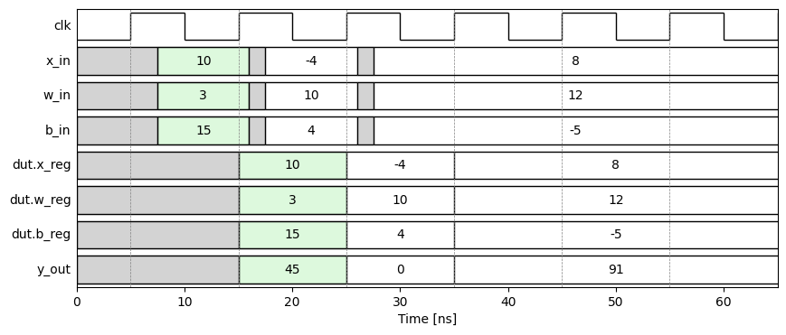
Visualizing the Timing Diagram

Once the simulation is complete, it will create a Value-Change Dump or VCD file with the trace of all the inputs. You can then visualize that in jupyter notebook.

We can see that if the inputs w, b, and x are valid on the rising edge of clock cycle n, the output, y, will be valid before the rising edge of clock cycle n+1. Hence, the latency is one clock cycle. The diagram highlights the inputs, intermediate variables, and output for one of the inputs driven by the testbench.