Using Multiple Stages

A Polynomial Example

The simple function we started with could be computed in a single clock cycle and easily meet timing. In many cases, the function we need to compute takes multiple clock cycles. To illustrate, consider implementing a quadratic function of the form:

   y = w2*x*x + w1*x + w0

where the coefficients w0, w1, and w2 are fixed and x is an input. To make this simple, suppose that all the values are 16-bit signed integers (so there is a chance of overflow).

This function may be hard to compute in a single clock cycle. For example, we have to first compute the square x*x, multiply it by w2 and add it to the other terms. So, in a single clock cycle we would need to complete at least two multiplies and two additions. The propagation delay may be too large.

Dividing the Function over Multiple Stages

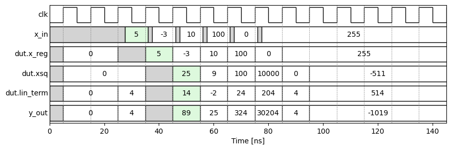
To implement this more complex function, we perform the operations over multiple stages. This function is implemented in hwdesign/demos/basic_logic/poly_fun.sv. Within this code, you can see three stages:

• Stage 0: Register the input x_reg <= x
• Stage 1: Compute and register the square xsq <= x*x and the linear term lin_term <= w1*x+w0.
• Stage 2 (combinational): Compute the output: y = w2*x + lin_term. This output is not registered to avoid additional delay.

So, if the input x is valid in on the positive edge of clock cycle n, the output y is valid on the positive edge clock cycle n+2. We say that the operation has a latency of 2.

Running the Simulation

As in the simple function example, we can run simulate the module with a testbench by opening a terminal, activating the virtual environment, and running:

    (env) sv_sim --source poly_fun.sv --tb tb_poly_fun.sv

This will generate a large directory sim with the simulation outputs including a file sim/dump.vcd with the VCD traces.

Viewing the Timing Diagram

Then, go to the jupyter notebook to see the timing diagram: