Timing — the loosely-timed model and its cosim calibration
This is the capstone page of the VMAC example: the other pages build the accelerator and prove it computes the right numbers; this one is a timing study. It takes the VMAC accelerator fed commands over an AXI-MM command queue and asks a harder question than “does it compute the right numbers” — does Waveflow’s loosely-timed simulation predict the right timing, where exactly does it stop being faithful, and can a cosim calibration close the gap?
The answer is a named result — bus utilization ≠ latency — framed in the standard comp-arch vocabulary for what the simulator is (a loosely-timed (LT) transaction-level model), and then corrected: a Vitis RTL cosim sweep calibrates the LT model so its latency tracks real hardware. The headline figure is committed and regenerates with no Vitis.
The system
One host, one accelerator, one shared memory, over a single m_axi master:
   host ──AXI-MM command queue──▶ VMAC ──m_axi (gmem)──▶ shared memory
 (vmac_host.py)                 (vmac_queue_sim.py)        A | B | Y regions
The host enqueues commands; VMAC dequeues them, reads its operand matrices A
(and B) from memory over m_axi, computes, and writes the result Y back to
the same bundle. Modeled in
examples/vmac/vmac_queue_sim.py and
examples/vmac/vmac_host.py; the
synthesizable kernel is
examples/vmac/vmac_compute_impl.tpp.
Two commands, same opcode
Both scenarios run the same inner_prod opcode (R = A·conj(B)) at PF=1 on
4×4 operands, 100 MHz — they differ only in where B points:
anorm—b_addr == a_addr.BaliasesA(an auto-correlation / norm). The kernel derives a loop-invariantab_eqflag froma_addr == b_addrand fillsb_lanefroma_laneinstead of issuing a second read burst.abcorr—b_addr != a_addr. The ordinary case: bothAandBare read.
ab_eq is a runtime flag, so HLS fixes one static II for the loop at the
worst case (b-read present). It does not reschedule shorter when ab_eq holds — it
only predicates whether the AXI transaction fires. That is the whole study:
same cycle count, B’s bus beat suppressed.
The starting point: a transaction-gated LT sim
The SimPy run logs a source-agnostic timeline — per-command memory
transactions (rw/name/addr/nwords/tstart/tend), latency, read-word
counts, and the command-queue occupancy. The Stage-1 LT model issues one
whole-matrix block per operand (16 words in a single bus transaction) and made a
command’s latency the sum of its transfer blocks — transaction-gated. Its
prediction:
| scenario | read words | latency (naive LT) |
|---|---|---|
anorm (ab_eq) |
16 | 630 ns |
abcorr |
32 | 940 ns |
Half the reads and lower latency for anorm — the intuitive “fewer reads →
faster” reading. Both halves of that turn out to be wrong about latency, and the
RTL cosim is what exposes it.
What the RTL actually does
Vitis RTL cosim measures the truth. At 4×4 the kernel takes 347 cycles for
both scenarios — anorm and abcorr are identical in latency, and anorm
genuinely issues half the read-bus words:
| scenario | read words (RTL) | latency (RTL) |
|---|---|---|
anorm (ab_eq) |
16 | 3470 ns |
abcorr |
32 | 3470 ns |
Two distinct errors in the naive sim fall out:
- Ordering. The sim said
anormis faster; the fixed-II RTL says equal latency, freed bus — eliding B’s read frees bandwidth, it does not shorten the pipeline. (bus utilization ≠ latency) - Absolute scale. The sim’s 630–940 ns sit ~5× below the RTL’s 3470 ns: the block model counts transfer time, not the kernel’s pipeline depth.
Both are the same root cause — a transaction-gated model can’t see a pipeline whose latency decouples from the transaction count.
The fix: cosim-calibrated II-decoupling
The repair is II-decoupling (TLM’s LT→AT escalation — add just enough timing structure for the question at hand): make a command’s latency the kernel pipeline schedule instead of the transfer sum,
latency_cycles ≈ depth + II · trips, trips = n_rows · ⌈n_cols / PF⌉
while still issuing the bus transactions for occupancy. Latency becomes
II-driven (depends only on trips, so anorm latency == abcorr latency — the
fixed-II behaviour) and occupancy stays transaction-driven (anorm still issues
half the reads). It lives entirely in the sim timing model
(VmacAccel.run_proc); the byte-exact golden
execute() is untouched.
Calibration is a sweep, validated on a held-out point
Fitting (depth, II) to the single 4×4 point would be tautological — one free
parameter against one measurement always matches. So
vmac_cosim_sweep.py cosims four
sizes spanning distinct trip counts and commits the swept RTL cycles to
calibration/vmac_calibration.json:
| size | trips | RTL cycles | RTL latency |
|---|---|---|---|
| 4×4 | 16 | 347 | 3470 ns |
| 6×6 | 36 | 725 | 7250 ns |
| 8×8 | 64 | 1258 | 12580 ns |
| 8×16 | 128 | 2435 | 24350 ns |
vmac_calibrate.py fits the model on
three of them and validates the prediction on the held-out fourth:
- Fit on {4×4, 6×6, 8×8}: depth = 42.7 cycles, II = 19.0 cycles/trip (R² = 1.0000).
The data is cleanly linear in
trips;II ≈ 19is the memory-gated inner-loop interval,depth ≈ 43the fill/drain + reduce-loop overhead. - Held-out 8×16 (trips 128): predicted 2472 cycles vs actual 2435 — 1.54 % error. Leave-one-out over all four sizes stays ≤ 3.6 %.
The same (depth, II) predict an un-fit configuration — that is what makes this a
calibration, not a curve-trace. (It also seeds the DSE vision: the calibrated LT
model now predicts un-cosim’d configs fast.)
The corrected result
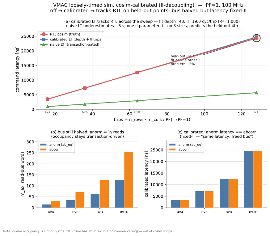
The calibrated sim now reproduces both facts the naive model missed, while keeping the one it got right:
| naive LT | calibrated LT | RTL | |
|---|---|---|---|
anorm latency (4×4) |
630 ns | 3464 ns | 3470 ns |
abcorr latency (4×4) |
940 ns | 3464 ns | 3470 ns |
anorm vs abcorr latency |
anorm faster ✗ | equal ✓ | equal |
anorm read words |
16 (half ✓) | 16 (half ✓) | 16 (half) |
- Panel (a) — off → calibrated → tracks RTL: the naive curve underestimates ~5×; the calibrated curve sits on the RTL line across the whole sweep, including the held-out 8×16 point it was never fit to.
- Panel (b) — bus still halved:
anormreads half ofabcorrat every size. Occupancy stayed transaction-driven; the II-decoupling only touched latency. - Panel (c) — fixed-II: calibrated
anormlatency ==abcorrlatency at every size — the “same latency, freed bus” result, now correctly modeled.
The named teaching result stands and is now quantified: ab_eq frees the
read-bus but does not shorten the pipeline — and on a shared interconnect that freed
bandwidth is exactly what another master (a CG matmul tile) would consume. The full
numeric writeup is the committed
calibration/vmac_calibration.json
and timeline/sim_sweep.json.
What this says about the model (loosely-timed TLM)
Waveflow’s simulator is a loosely-timed (LT) transaction-level model in the SystemC TLM-2.0 sense: each transfer is a single timed block that holds a capacity-1 bus resource for its whole duration, and concurrent masters serialize on it (an implicit arbiter). This is accepted, standard practice — LT is how industry virtual platforms run fast — not a Waveflow shortcut. Framing the result, and its repair, in that vocabulary is the point of the example.
What LT captures faithfully here:
- Total interconnect occupancy (Σ of held block durations).
- Multi-master contention / arbitration (serialization on the capacity-1 bus).
- First-order, burst-granular memory-access timing — including the
ab_eqread-word halving, which the sim gets right in every mode.
What LT abstracts away (the boundary):
- Sub-transaction interleaving / exact beat ordering — a block is contiguous, never “every other cycle.”
- Consequently latency is mispredicted wherever it decouples from transaction
count — the pipeline-depth and
ab_eqcases above.
Fidelity per validation target, and how the calibration moves it:
| Target | Fidelity under the LT block model |
|---|---|
| Queue occupancy | Robust — command-level granularity; the block model is plenty fine |
| Per-burst / total memory occupancy | Robust — the bus resource sums it correctly |
ab_eq latency & absolute latency |
Recoverable — closed by the (depth, II) cosim calibration |
| Sub-transaction ordering / fine contention | Irreducible gap — the block can’t say who’s on the bus which cycle |
Escalating from transaction-gated to II-parameterized latency is Waveflow’s analog
of TLM’s LT→AT escalation: the calibrated (depth, II) add just enough timing
structure to answer the latency question, no more — sub-cycle ordering remains
deliberately out of scope.
Scope note. Queue occupancy is a sim-only quantity here: the cosim kernel has an
m_axibut no command ring, so the calibration validates per-burst memory timing and theab_eqread-word result against RTL; occupancy is reported by the sim alone and not fabricated for cosim.
The committed figure (regenerates without Vitis)
The figure is rendered by
examples/vmac/vmac_figures.py from the
committed sweep timeline alone —
timeline/sim_sweep.json, which
carries the naive, calibrated, and RTL latencies per size — no Vitis, no cosim
re-run, no VCD read. That is the “committed figure” property: the docs build never
needs the toolchain.
cd examples/vmac
python vmac_calibrate.py         # print the fit + held-out validation (reads the calibration JSON)
python vmac_queue_sim.py         # re-emit timeline/sim_timeline.json + timeline/sim_sweep.json
python vmac_figures.py           # re-render docs/examples/mmqueue/images/sim_vs_cosim.svg
python vmac_figures.py --check   # render to a temp file, byte-compare vs the committed SVG
The SVG is deterministic (a fixed svg.hashsalt, no embedded timestamp, mirroring
shared_mem_figures.py), so a
re-render is byte-identical when nothing changed. images/sync_status.json records
the source-JSON hash and the SVG hash, a cheap staleness signal a docs lint can check
without re-running anything. The RTL truth was captured once by the Vitis-only
vmac_cosim_sweep.py (and the 4×4
headline by vmac_cosim_stage3.py) and
committed.
Where this sits
- The VMAC example overview — the rest of the walkthrough this timing study caps: the command schema, the one-golden model, the SimPy sim, the generated top, and the RTL conformance whose cycle counts feed the calibration here.
- The C and RTL simulation page — where the committed RTL cycle counts this calibration fits come from.
- The Histogram with shared memory example — the previous step in the
examples progression, where the
m_axishared-memory pattern is introduced, with its own RTL cosim and committed timing figures.