Viewing Timing and Bursts

The RTL simulation page produced a cosim waveform and a burst report. This page turns those into two pictures — the multi-buffer burst layout and the transaction timeline — and documents how the figures are committed and refreshed. Both are rendered by shared_mem_figures.py from the cosim burst report (vcd/burst_info.json), which is itself regenerable from the committed vcd/dump.vcd with no Vitis run.

The burst layout

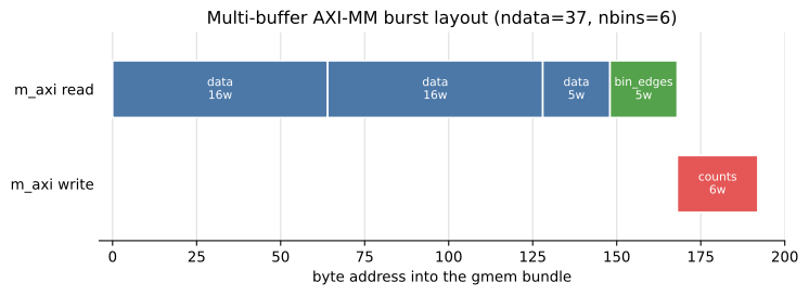
This is the figure unique to the shared-memory example — the visual payoff of the multi-buffer m_axi story. It shows where, in the one gmem bundle, each buffer lives and how the m_axi master bursts it, for the ndata=37, nbins=6 vector:

• data (read, 37 words from byte 0) is split into three bursts — 16 + 16 + 5 words. The m_axi interface has a maximum burst length (16 words here), so a 37-word read becomes three back-to-back bursts rather than one 37-beat transfer. This splitting is automatic; the kernel just asked for 37 elements.
• bin_edges (read, 5 words from byte 148) is one short burst, immediately after the data region — 5 words because nbins-1 = 5 edges define 6 bins.
• counts (write, 6 words from byte 168) is the one write burst — nbins = 6 count words, after both input regions.

Read the address axis left to right and you are reading the memory map the command chose: data_addr = 0, bin_edges_addr = 148, cnt_addr = 168, back-to-back because the allocator placed them in that order. Two element types (float reads, uint32 write), three buffers, one bundle — exactly what the example set out to exercise.

The transaction timeline

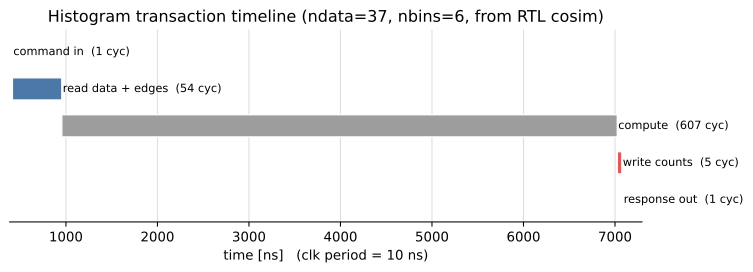
This is the same transaction over time, broken into phases and annotated with cycle counts (the clock period is 10 ns). It reads as the execution model did: command in → read the inputs → compute → write the counts → response out.

The shape is worth noting: compute dominates. The two m_axi reads finish in tens of cycles, and the write is a handful more, but the binning loop over 37 samples is hundreds of cycles — so the memory traffic is a small slice of the transaction. That is a real and useful reading: for this kernel the bottleneck is the datapath, not the bus, which is why the multi-buffer burst efficiency (the read splitting above) costs so little of the total. A heavier-data / lighter- compute kernel would show the opposite balance.

The cosim timeline is what the SimPy model was approximating; here the phase boundaries and the burst latencies are measured from real synthesized RTL.

How the figures are committed

The docs site cannot run Vitis or SimPy at build time, and committing a freshly generated figure on every run would churn binary blobs in git constantly. So the figures live in three places, with a deliberate promotion between them:

Location	Tracked?	Role
examples/shared_mem/results/*.svg	gitignored	generated each render — never committed
docs/examples/shared_mem/images/*.svg	committed	the stable assets these pages embed
docs/examples/shared_mem/images/sync_status.json	committed	provenance: each figure’s source path + content hash

The render steps (generate_burst_diagram, generate_timing_diagram) write into results/; a separate SyncDocsFiguresStep copies them into images/ on demand, driven by an explicit manifest (results/... → docs/.../images/...). The sync never copies by guesswork — the manifest is the reviewable mapping, and the copy is a normal git diff you choose to commit.

Refreshing the figures

The whole workflow runs from hist_build.py:

cd examples/shared_mem
python hist_build.py --through sync_docs_figures

That renders both SVGs from vcd/burst_info.json and syncs them into images/. If burst_info.json is missing, the render step regenerates it from the committed vcd/dump.vcd — so a routine figure refresh needs no Vitis, only matplotlib (already required by the example’s timing utilities).

To refresh against new hardware behavior — after changing the kernel, the buffer sizes, or the test vector — regenerate the cosim artifacts first, then sync:

python hist_build.py --through extract_bursts --trace-level port  # new dump.vcd + burst_info.json (needs Vitis)
python hist_build.py --through sync_docs_figures           # re-render + sync
git diff docs/examples/shared_mem/images/                        # review, then commit

Because the SVGs are rendered deterministically (a fixed svg.hashsalt, no embedded timestamp), a re-sync produces a byte-identical file when nothing changed — so the git diff is empty unless the hardware behavior actually moved. sync_status.json records each figure’s source content hash at the last sync, a cheap staleness signal a docs lint can check without re-running anything.

Next

This is the last page of the shared-memory walkthrough. For the broader references, see:

• Build System — the BuildDag / BuildStep reference behind the figure workflow.
• Interfaces — the AXI-MM / stream abstractions.
• The examples index — the five-pattern progression this example sits in.