A memory reached three ways
Sharing memory between concurrent tasks arises in a multitude of applications — capture buffers, scoreboards, and storage of intermediate values. As the memory guide describes, there are three ways to share memory between hardware modules:
- External memory, typically DDR, that exists on the board and reaches the programmable logic over an AXI-MM interface.
- A ping-pong buffer (PIPO), which transfers blocks with a synchronization mechanism built in.
- A dedicated BRAM (Block RAM), instantiated in the top-level design in the programmable logic.
This example demonstrates implementing, modelling and using a BRAM, where two hardware modules share one true-dual-port memory. For shared DDR see the histogram example; for the ping-pong buffer, the interleaver example.
The interface itself is documented in BRAM — memory between modules; this page set is the worked example that uses it.
Why a dedicated BRAM?
A BRAM can be given dedicated access to a small number of hardware modules. DDR usually has to be shared with other modules and with the PS, which can add substantial delay.
A PIPO is also typically built from a two-port BRAM, but it comes with a synchronization mechanism you do not choose, and it requires one module to write a different buffer segment than another reads. A BRAM gives you the memory and leaves the correctness argument to you — which is the whole subject of this example.
The example
Two hardware modules share one BRAM, and the memory is reached three ways — which is where the name comes from, and which lines up with the three access cases that every Waveflow interface is organised by:
| transaction | access case | what it costs |
|---|---|---|
WRITE |
a timed transfer into the memory | 1 access per element, II=1 |
COMPUTE |
in place — no transfer at all | 2 accesses per element, II=2 |
READ |
a timed transfer out of the memory | 1 access per element, II=1 |
WRITE and COMPUTE go through the same port on the same task, so the only thing that differs
between them is the access shape. That makes the II a measurement in one waveform rather than an
argument, and it is why this example has two opcodes instead of two examples.
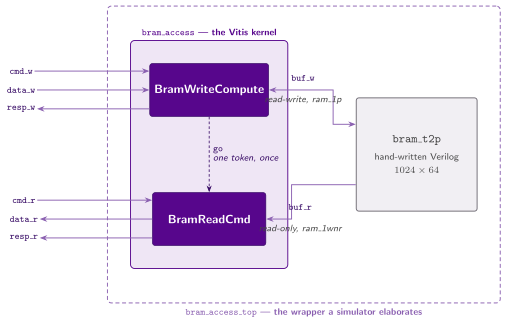
The nesting is the point. The memory is outside the kernel and inside the wrapper, because a
memory shared between two tasks has no expression inside a Vitis kernel at all —
the guide has the evidence,
including the two things Vitis does instead when you try. Every transaction takes a command and
answers with a (tid, status) response: a write has no return path of its own, and a refused read
returns zero words, which on a stream is indistinguishable from “not yet”. The messages are declared
once as schemas, and the C++ headers the kernel compiles against are generated from them.
What you will learn
- How to create a memory and connect two
HwModules to it through aBramIF— and why it is registered withadd_rtl_ifrather thanadd_if. - How to move a vector into it, and how to compute over it in place without inventing a transfer — and what declaring a port read-write costs you in cycles.
- How to read and write it concurrently, and what actually guards the hazard — which is not the thing the memory’s own Verilog appears to promise.
- How to run the design in Python simulation and record its timing.
- How the read path’s fill is modelled, and why that number must never be typed into Python.
- How to run an RTL simulation in which the memory is the real hand-written Verilog, with no BFM standing in for it.
- How to verify throughput, overlap and the in-place cost from a timing diagram built out of the RTL trace.
Once you have this example, the same structure is what the RF shot buffer is built on.
The pages
- Python model — the three transactions, the schemas, the two task bodies, and the top level with the memory beside it.
- Python simulation — running it, the test vectors, and recording the timing.
- Code generation — the kernel,
bram_t2p.v, and the wrapper that joins them. - RTL simulation — running XSI, and producing the trace.
- Reading the trace — the activity diagram, the hazard scan, the in-place cost, and the comparison to pysim.
See also
- BRAM — memory between modules — the interface, the evidence for why the memory cannot be inside a kernel, and the addressing convention.
- A module realized as Verilog — the
rtl_module()hook, the port-name chain, and the latency single-source rule. - Free-running composite — where the wrapper
fits, and what
csynthdoes not count.