Timing in the pysim
The interleaver’s loosely-timed pysim charges modeled delays and lets backpressure emerge from the bounded FIFOs between stages — fast, functional, no toolchain. This page is what it measures and the pipeline-activity plot it produces; the next page measures the actual RTL timing and compares the two (they agree to ≈1%).
What the pysim measures
The pysim never runs the RTL. Each stage’s cost is a loaded model:
- the bus law — each
m_axitransfer’s cost,nwords + (num_trans − 1)cycles per read (BusCalib); - the mem-stream residuals — the reader’s ≈15-cycle and writer’s ≈22-cycle own control cost, on top of the bus term (the mem-stream residual);
- the compute loop model — the gather’s
cycles = n(the timing model).
Each free-running stage records a per-firing fire_log, and the whole run lands at 300 cyc/job.
The pipeline at a glance
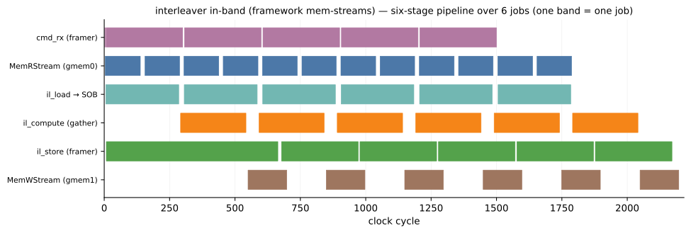
Every stage on one cycle axis, six jobs, rendered straight from the pysim fire_logs. Reading it top to
bottom is reading the dataflow — one job descends the stack:
cmd_rxreceives theInterleaverCmdand frames two reads (P then X) for the reader.MemRStream(gmem0) — the two bands per job are those two reads; it is busy almost continuously, and it is the bottleneck (movingPandXover one bus).il_loadlandsPandXinto the on-chip stream-of-blocks.il_computeruns the gatherY[i] = X[P[i]]— its band has visible slack (256 of the ≈300-cycle job), the one stage this design calibrates itself, not on the critical path.il_storeframes the writer’s stream[MemWCmd | Y].MemWStream(gmem1) burstsYto memory and echoes the done.
The bands are occupancy, not work. A band is a stage’s firing window — from when it starts a firing to
when it commits — so for a free-running stage it includes time spent stalled on backpressure, not just
its own compute. cmd_rx is the clearest case: it does about 5 cycles of real work (build two
commands), but its steady-state band fills the whole ≈300-cycle job — because it cannot dispatch the next
job’s commands until MemRStream has taken this one. The long bar is throttling, not effort. The reader’s
own two bands, by contrast, are close to solid work: it is the bottleneck, so nothing downstream throttles
it. (The thin seam between consecutive bands is only a legibility device, so you can count the jobs.)
The build DAG
How to regenerate it. The figure has a two-rung build DAG, run through the standard CLI:
python examples/interleaver/interleaver_figures.py               # pysim -> timeline -> figure
python examples/interleaver/interleaver_figures.py --list-steps  # interleaver_source, pysim, figures, rtl_timing
InterleaverPySimStepruns the fully-calibrated pysim, checks the gather golden, and writes the per-stage timeline toresults/interleaver_pysim.json;InterleaverFiguresStepconsumes that artifact and renders the SVG — it does not re-run the sim. The source is the pysim timeline: deterministic and toolchain-free, so the committed SVG regenerates anywhere (including CI, where Vitis/xsimare absent) and a re-run is a no-op unless the timeline moved. Each stage’sfire_log(its per-firing(start, end)windows) becomes oneActivityDiagramlane:lanes = [] for stage, label, colour in stages: # each firing window -> a run of active cycles (a small seam trimmed off the end, for legibility) runs = [np.arange(round(s), round(e) - seam) for s, e in stage.fire_log] lanes.append((label, np.concatenate(runs), colour)) ad = ActivityDiagram(lanes, time_unit="cycle") fig, _ax, _ = ad.plot(mode="band", ...) # activity bands, not per-transition value boxes
The same ActivityDiagram could instead be fed an RTL trace’s component_firings (the ground-truth view
mem_copy uses), but the committed figure stays on the pysim timeline for exactly
the reason above — and the RTL timing is where the next page goes, to check it.
Next: does it match the RTL?
The 300 cyc/job is the model’s number. RTL timing and the comparison measures the real RTL cadence from a trace and puts the two side by side.
See also
- The timing model — the per-stage models the pysim charges.
- RTL timing and the comparison — the RTL measurement and the cadence table.
- Activity Diagrams — the renderer behind the figure.