Visualizing timing

The pysim and RTL rungs agree on the steady-state period — about 183 cycles per job. They agree because mem_copy composes two calibrated framework components — MemRStream / MemWStream and the bus model — and Waveflow ships their timing parameters for this platform (zynq7020_bfm_100mhz), so the loosely-timed pysim reproduces the RTL number with no manual tuning. (How those infra models are built and fit — a general, design-independent facility — is the calibration guide; mem_copy itself calibrates nothing.)

This page is about seeing that timing — how the stages overlap, which one is the bottleneck, and where every cycle of the period goes. That means tracing the RTL run and rendering it.

Tracing the run

To see inside the kernel — the two internal framed_word FIFOs (cmd and copy_data) that wire the three tasks, and both m_axi bundles — we pull those signals out of an RTL run by exact name. That is general Waveflow machinery, the four trace steps:

python examples/mem_copy/mem_copy_build.py --through extract_bursts

That produces mem_copy_trace.vcd (the waveform), mem_copy_trace.json (the net-name manifest), and mem_copy_timing.json (a per-firing timing table). A fifth step, timing_figures, renders the pictures below.

How these are drawn. The two timeline figures below come from a reusable renderer, ActivityDiagram — a sibling of the TimingDiagram that swaps per-transition value boxes for activity bands and an optional occupancy sub-panel, so it stays legible across thousands of cycles. Any design can build the same views from its trace: ActivityDiagram.from_trace(bt, spec) walks a manifest’s channels and ports into lanes; the example’s timing_figures step supplies only mem_copy’s own lane spec. The third figure (per-firing spans) is a bar chart off the timing table, not a lane-on-time-axis plot, so it stays example-specific.

The run at a glance

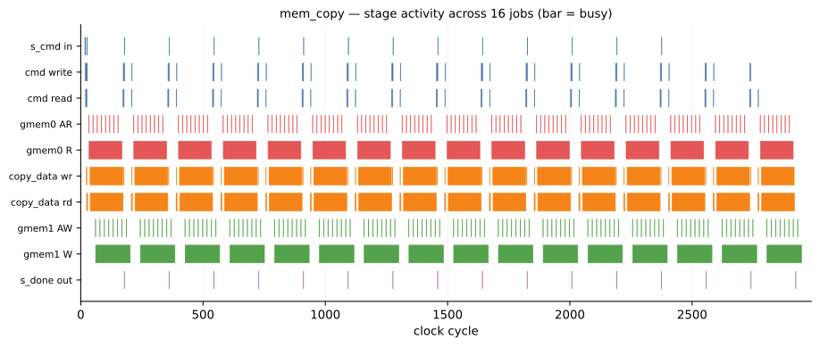
Stage activity across the whole run

Every stage of the pipeline on one cycle axis, 16 jobs. Three things are visible before any analysis: the 183-cycle cadence; that gmem0 R (reads) and gmem1 W (writes) are busy simultaneously rather than in turn, so the design really is pipelined; and that the writer’s green band is nearly continuous while the command lanes at the top are almost entirely idle. The writer is doing something close to all the work.

The per-firing table

Each free-running stage fires once per job, and the ExtractBurstsStep writes one row per firing:

{"component": "mem_w_stream_framed_done_task", "index": 8,
 "start": 1488, "end": 1670, "span": 183,
 "nwords": 128, "num_trans": 8, "blocked": 0}

span is the firing’s true occupancy — first input handshake to ap_done, not its last output beat, because the writer’s m_axi stores are posted and keep draining after s_done (why). blocked is cycles its output channel sat at capacity, read from the FIFO occupancy counters rather than a write enable (why).

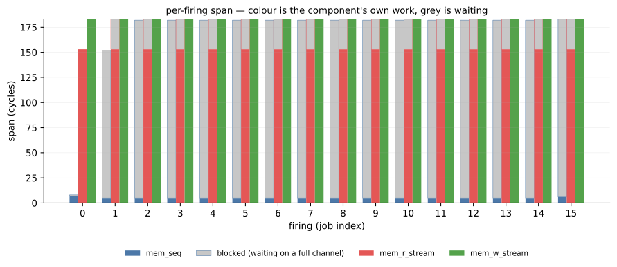
Per-firing span, split into own work and waiting

Colour is the component’s own work, grey is waiting on a full channel — and the bottleneck needs no arithmetic to spot. The writer is solid green at 183 on every firing: busy the entire period. The reader is 153 on its first firing, then 153 + 30 grey. The sequencer is ~5 cycles of work against ~175 of waiting — it finishes a command almost immediately, then sits behind everything downstream. So the writer is the bottleneck, 100% utilised at 183 of a 183-cycle period; the reader’s 30 grey cycles are it waiting on a writer still draining — emergent congestion, not a property of the reader.

Where the 30 cycles are

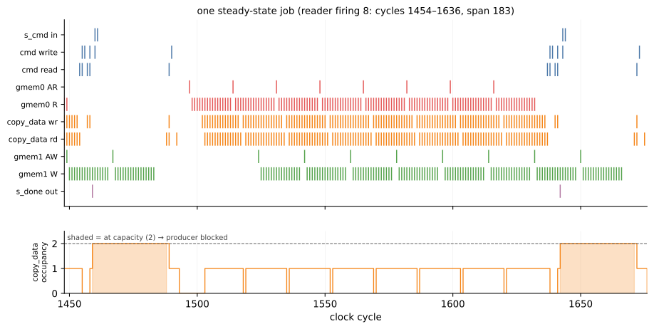
One job, beat by beat, with FIFO occupancy

One steady-state firing. The lower panel is the copy_data FIFO’s occupancy, and the shaded band is it at capacity — the reader blocked, unable to hand over its descriptor words, because the writer has not finished draining the previous job. The reader’s gmem0 AR bursts (top panel) only begin after that band clears. Look at the far right: s_done out fires, and gmem1 W keeps going for another ~24 cycles — the posted-write drain, the reason a firing ends at ap_done, not at s_done.

And the pysim matches — for free

Everything above is the RTL. Run the pysim with the same shipped calibration and it reproduces the 183-cycle period to 0.0% — the fast, toolchain-free model predicts the slow RTL.

And mem_copy calibrates nothing to get this. It composes only reusable infra — the MemRStream / MemWStream adaptors and the m_axi bus — whose timing models are a (component, platform) property that ships with Waveflow for supported platforms. mem_copy loads them and inherits the right timing; there is no sweep, no fit, no per-example calibration step. That is the payoff of the two-level design: the shared bus and mem-stream models are fit once (they happen to have been measured on mem_copy, behind the scenes in calibrate_platform.py), and every accelerator on the platform reuses them.

Where those models come from, and how you’d fit one for a custom component of your own, is a general facility documented in the calibration guide — and worked end-to-end, for a design that does add a custom component, in the interleaver example.